")
")
How do we simulate stock price movements? (Part I)
In our previous article, Deep Hedging --- Trading Vanilla Options with Neural Network, we mentioned that in order to access the overall risk profile of our hedging algorithm, an extensive amount (e.g., \(10^6\)) of simulated stock price trajectories are needed. These trajectories could each represent a market projection consists of a particular set of random variables. As we never know the future shape of a market, it is necessary to cover as many random scenarios as possible. We cannot just use historical paths to mimic what will happen in the future, as there is always something unprecedented. Therefore, what we always do in practice is, first, to get the parameters’ values for the stochastic model(s) we think is suitable for our purpose, which is called the model calibration process. Then we simulate many possible future scenarios (trajectories) of the time series we are interested in. Finally, we will analyse these scenarios and conclude what results from our algorithm will possibly get in the future.
Here we will talk about several most common stochastic models for financial time series analysis.
Brownian Motion: The History
Brownian motion is not directly used in financial modelling nowadays, but it is the foundation of everything.
In 1827, Scottish botanist Robert Brown first described the random fluctuations of a particle’s position suspended in a fluid. Almost eighty years later, in 1905, Albert Einstein published an article on Annalen der Physik (English: Annals of Physics) to explain the motion as being moved by individual water molecules and gave mathematical formulae. Until then, people finally have a theory for predicting naturally occurring random events. Actually, this is Einstein’s first major scientific contribution, and 1905 is also called his miracle year.
The first description of something related to the random movements of assets’ prices is five years before Einstein. A French mathematician Louis Bachelier submitted his doctoral thesis Théorie de la speculation (English: Theory of Speculation) in 1900. Louis stated that if there are predictable patterns of financial assets’ prices, speculators will find the patterns and exploit them, thereby eliminating them. Bachelier’s ideas were just far ahead of his time, where there was hardly anyone who tried to apply mathematics to an unrelated area called finance. Therefore, his piece of work has been ignored for more than sixty years. Until 1965, economist Paul Samuelson published an article called Proof That Properly Anticipated Prices Fluctuate Randomly, which picked up Bachelier’s thoughts and first provided the mathematical foundation for claiming that if the market is well-informed, all forecastable changes have already reflected in the current prices. The remaining drivers for price movements are only random factors. This is also later become known as the efficient-market hypothesis.
Since then, people started developing stochastic models for financial time series simulation.
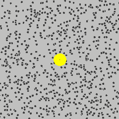
Brownian Motion: Random Walk and Wiener Process
English statistician Sir Francis Galton invented Galton Board to demonstrate the central limit theory.
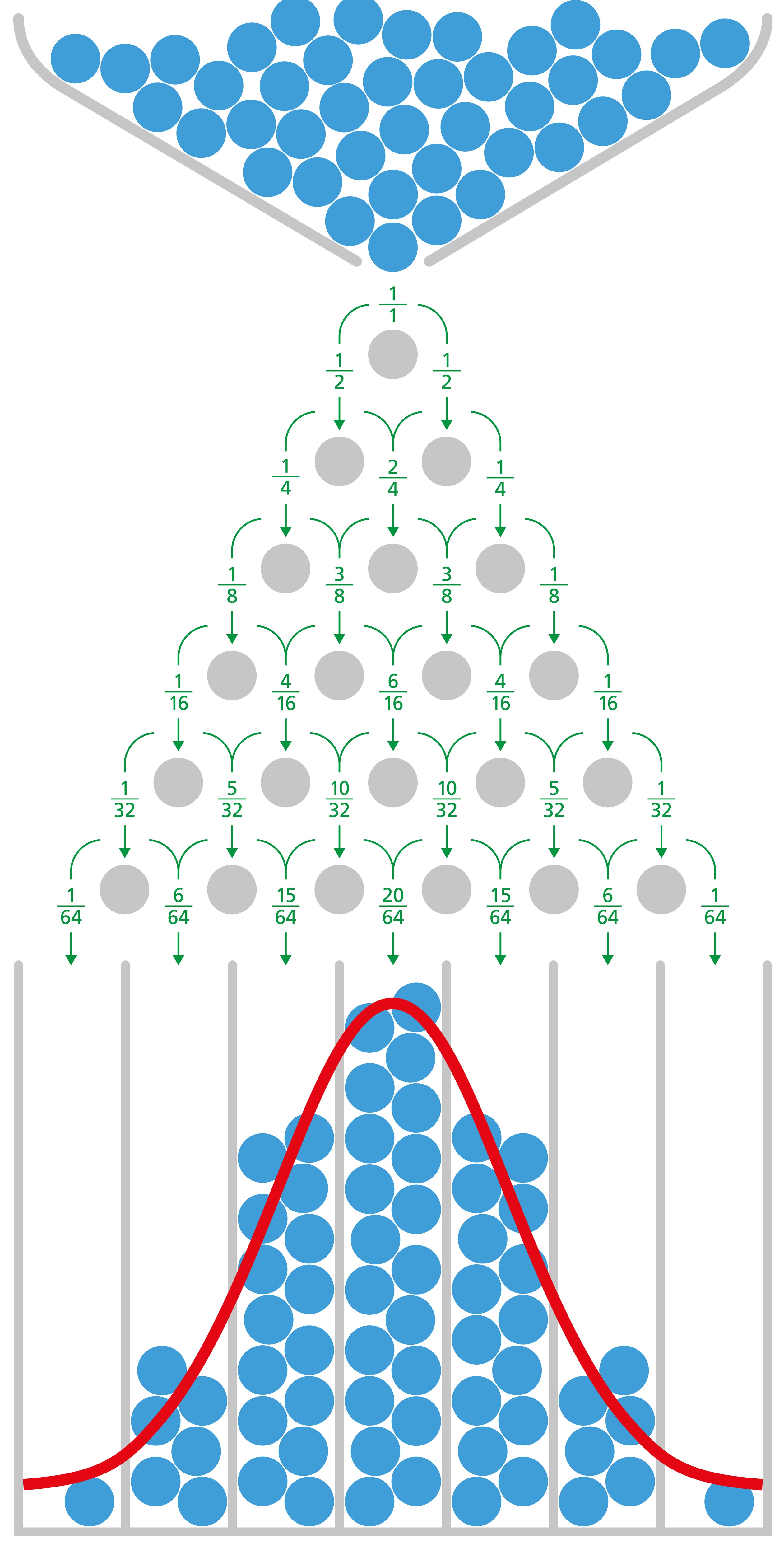
We consider it takes six steps to reach the bottom grid for each blue ball in the picture. At each step, it can only go left or right with an equal probability of 50%. We can see that most balls end up in the middle column, and the first and last columns have the fewest balls. This can be considered a random walk of six steps, where each step is independent but with identical possibilities and probabilities. From the central limit theory, we know the final positions of balls should be normally distributed.
If we rotate the picture 90 degrees anti-clockwise, imagine it is a particle travelling from point (0,0). For every step, it is also taking independent but identical distributed steps. If the size of each step is infinitely small. One possible path of travel will be something like in the picture:
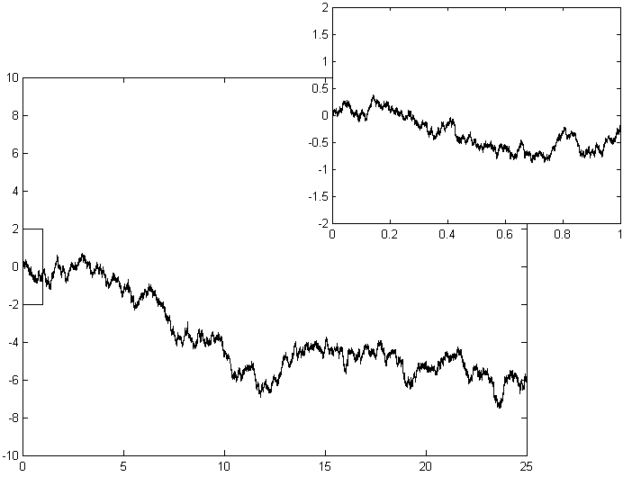
This is called a Wiener process. It is equivalently to a random walk with infinitely small steps. We also call it standard Brownian motion. It can be used to model a particle’s movement as overserved by Robert Brown.
Brownian Motion with Drift
Mathematically, a Brownian motion with drift S(t) is the solution of a stochastic differential equation (SDE):
\(dS(t)=\mu dt+\sigma dW(t) \),
with initial value \(S(0)=s_0\). Take direct integration, we get:
\(S(t) = s_0 + \mu t + \sigma W(t)\)
Here, \(W(t)\) represents is a Wiener process discussed above.
\(s_0\) is the very first price of this stock. One can arbitrarily define this value or take a real value from the market. For example, IBM stock price at the end of 21/05/2021 is USD 144.74. Then we define what \(S(1)\) means. If it means IBM stock price at the end of 24/05/2021, then \(t\) is the sequential number of days, or it could also be months, hours, minutes, or whatever time frame.
\(S(t)\) is representing the price of a stock at time \(t\) , which is a combination of a constant \(s_0\), a linear function of time \(\mu t\) and a scaled Wiener process \(\sigma*W(t)\).
We usually consider \(\mu\) as defining the long-term trend of the share price, and it is referred to as the risk-free interest rate. \(\sigma\) is effectively the volatility of the share. A larger value of \(\sigma\) indicate the stochastic factor (Wiener process) have a bigger fluency, so share prices are more likely to fluctuate.
So far, we have a pipeline to simulate one trajectory of a financial time series with a period of, for example, ten days:
- Generate ten independent values from a standard normal distribution.
- Calculate the values of the Wiener process \(W(t)\) for t = 1,2,3 … 10.
- Set the parameters values of \(s_0\), \(\mu\) and \(\sigma\).
- Calculate \(S(t)\) for t = 1,2,3 … 10, using those parameters and the Wiener process.
Instead of just one path, we should simulate a large amount of Wiener processes to represent many different random scenarios. And produce many simulated time series.
Geometric Brownian Motion
Someone may has noticed that method mentioned above has a fatal drawback while simulating financial time series. There is a possibility that \(S(t)\) become negative if \(\sigma\) is much larger than \(\mu\), which is not possible in real lie. Therefore, we should use Geometric Brownian Motion with SDE:
\(dS(t) = \mu S(t)dt + \sigma S(t) dW(t)\),
with initial value \(S(0)=s_0\). And we have:
\(S(t) = S(0) exp[(\mu - \frac{\sigma^{2}}{2})t+\sigma W(t)]\)
This is effectively modelling the return from a share \(\frac{S(t)}{S(0)}\) as an exponentiated Brownian motion., which is more sensible in the financial context, and \(S(t)\) will never be less than zero.
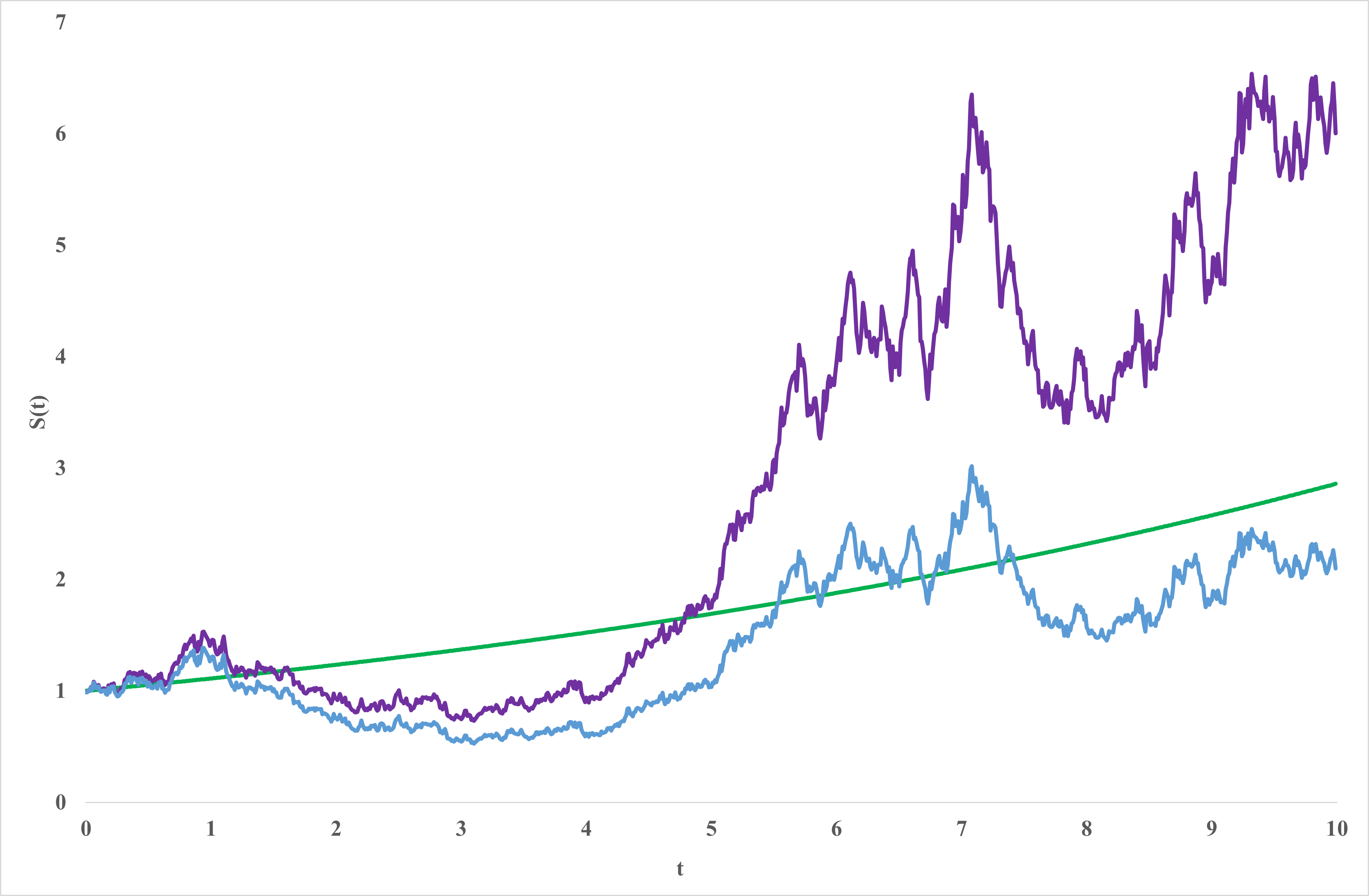
In this picture, purple line is the geometric Brownian motion process, the green line is the linear factor \(exp[(\mu - \frac{\sigma^{2}}{2})t]\) and blue line is the stochastic factor \(exp[\sigma*W(t)]\) . The parameter values are \(S_0 = 1\), \(\mu = 0.15\) and \(\sigma = 0.3\).
For the geometric Brownian motion model, the value of \(\sigma\) does not change no matter what the value of \(t\) is, indicating that the stock price volatility is always constant. We know from the intuition that this does not hold in reality, because during some periods (e.g., when significant political/economic change happens), stock prices fluctuate more than other times. So we have to add some randomness associated with the volatility of the asset price, which becomes the stochastic volatility models.
(To be continued)
Reference:
Einstein, Albert. "Über die von der molekularkinetischen Theorie der Wärme geforderte Bewegung von in ruhenden Flüssigkeiten suspendierten Teilchen." Annalen der physik 4 (1905).
Bachelier, Louis. "Théorie de la spéculation." In Annales scientifiques de l'École normale supérieure, vol. 17, pp. 21-86. 1900.
Samuelson, Paul A. "Proof That Properly Anticipated Prices Fluctuate Randomly." Management Review 6, no. 2 (1965).
https://en.wikipedia.org/wiki/Brownian_motion
https://en.wikipedia.org/wiki/Wiener_process
https://www.cantorsparadise.com/brownian-motion-in-financial-markets-ea5f02204b14
Hits: 4101