Deep Hedging --- Trading Vanilla Options with Neural Network

The first article discussed using neural network models for pricing and hedging financial derivatives could be dated back to 1994. Based on the Universal Approximation Property of neural networks, Hutchinson et al. (1994) proposed that learning networks could be valuable substitutes when conventional parametric methods fail. They also experimented with S&P 500 futures options data from 1987 to 1991.

After that, there were not many developments in this direction. We think the accessibility of powerful computing resources is one of the constraints, only made available to many industries and academics until recent years.

Deep Hedging was proposed in 2018. The writers are from JP Morgan and ETH. We have reasons to believe this neural networks based solution for pricing and hedging have already been imposed in the trading floor. 

Background and Assumptions

Assume you are the seller of a European call option, which means the option buyer could only exercise it at maturity. We set it to 30 days from now. During this period, you need to keep adjusting your holdings of the underlying asset to hedge your risks exposed in the option contract. If there is no trading cost and continuous trading (trade at every second) is possible, you will be guaranteed zero profits or losses at the end of the 30 days. However, this is nothing that will even happen in real life. So you will incur an overall loss at the termination, and the premium you charged when signing the contract reflected your expectation of this loss.

Limitations of the conventional Methods

With the conventional Black-Scholes-Merton (BSM) method, the initial price of an option, as well as the appropriate holding amount to hedging the option contract, can be calculated from formulae. However, for the whole theory to work correctly, there are three assumptions to be satisfied. First, trading is always cost-free. Second, people can buy and sell the underlying asset continuously. Third, price movements of the underlying asset follow Geometric Brownian Motion (GBM), which indicates every price change follows a log-normal distribution, and the variance keeps constant over time. The first two assumptions are obviously contrary to realism, and the third has also been proven impossible from many observations, such as fat tail and volatility smile. In addition, many people thought one major cause of the financial crisis in 2008 is our underestimation of the fat tail.

We have many better models for financial time series, and Heston is one of them. With Heston model, there are two stochastic factors associated with the underlying price and its variance. Here is the formula:

\[dS(t, S) = \mu S dt + \sqrt{v} S dW_1\]

\[dv(t, S) = \kappa (\theta - v) dt + \sigma \sqrt{v} dW_2\]

\[dW_1 dW_2 = \rho dt\]

\(W_1\) and \(W_2\) are two stochastic variables with standard normal distributions, and their correlation is \(\rho\). \(S\) represents price of the underlying asset with its variance \(v\). All other parameters are constant. 

If the underlying asset prices follow the Heston model in real life, then the BSM method would no longer validate how much to charge an option and how to hedge it. Not even mention the trading cost and trading frequency issues.

Deep Hedging has made its way to use a neural network model for calculating option premium and hedging strategies when the first and third assumptions of BSM could not be satisfied. The parameters in the model could also be optimized with different risk appetites or utility functions at the trade's decision. As for the trading frequency assumption, the model only assumes trading happens once a day.

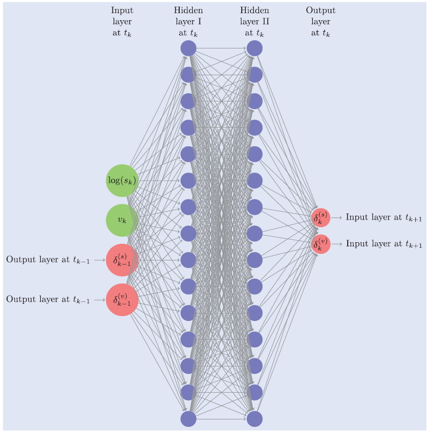
Structure of the Neural Network

The neural network structure for Deep Hedging is not very complex. It is not even considered "deep" if comparing with other popular network for computer vision. There are only two fully connected layers, with 15 neurons each. There are also an input layer and an output layer, which makes it four layers in total. 

Unique Loss Functions

One fundamental advantage of the neural network is the capability of utilizing various loss functions for different purposes. Speaking to financial derivatives, loss functions could represent someone's unique risk appetite or utility function. In other words, how he/she evaluates these cashflows according to his/her specific situations. Therefore, the loss function implemented by Deep Hedging is quite different from those adopted by image or language processing networks. The authors proposed two different types of functions. The first one is entropy risk measures:

\[\rho (X) := \frac{1}{\lambda}\log {E(e^{-\lambda X})}\]

\(\lambda\) is a constant number larger than zero, which considered as some risk appetite. As \(\lambda\) gets larger, an investor is willing to take more risks. The user of Deep Hedging could set his/her own value of \(\lambda\), which reflects specific risk tolerance, shareholders requirements and/or regulation constraints.

Another loss function is very commonly seen in regulation documents, which is expected shortfall:

\[\rho(X) := \frac{1}{1-\alpha}\int_{0}^{1-\alpha}VaR_{\gamma}(X)d\gamma\]

The logic behind is that one could first decide a probability that associated with normal scenarios, say 90%. Then calculate the expected losses if the remaining 10% extreme events happened, and consider this value as a baseline for risk preferences. If the value of \(\alpha\) is set to 99%, then the calculation is based on more extreme events than \(\alpha\) is 90%, so that expected losses are larger.  In practical experiments, we simulated \(10^6\) different possible trajectories of the underlying assets, using the model to hedge each of them and calculate the mean of the worst 1% termination losses. This could be the basis for determining the option premium.  In the formula, \(VaR\) is Value at Risk.

By linking the loss functions with the risk preferences, deep hedging is obviously more suitable for financial market participants. The regulation requirements are also easier to be met.

Summary

Deep Hedging started a new topic to find the non-linear relationship between prices of the underlying assets and its derivative instruments with neural networks. In this way, some unrealistic assumptions from the BSM method could be dropped. In addition, including risk preferences in the neural network training makes the algorithm much more applicable and explainable. 

However, there are also many aspects that could be improved with the current version of Deep Hedging. Instead of trading daily, there could be a mechanism to automatically make trading decisions when the underlying price reveals specific patterns. The neural network structure is also too naive, and recurrent neural networks may be better candidates. It would be exciting to see a combination of forecasting future underlying prices and generating hedging strategy simultaneously in an end-to-end neural network model. 

References

J. M. Hutchinson, A. W. Lo, and T. Poggio. A non-parametric approach to pricing and hedging derivative securities via learning networks. The Journal of Finance, 49(3):851–889, 1994.

H. Buehler, L. Gonon, J. Teichmann, and B. Wood. Deep hedging. Quantitative Finance,  19(8):1271–1291, 2019.

Notes: In the Deep Hedging paper, the authors actually used the combination of the underlying asset and a variance swap to hedge the option contract. As a variance swap is too complicated, it is not mentioned in this article.  In theory, using only the underlying is also feasible.

• Next